Persistent Homology

This guide covers the persistent homology pipeline in masspcf: going from point cloud data to persistence barcodes to stable rank functions, and using those functions for downstream analysis.

Background

Persistent homology is a tool from Topological Data Analysis (TDA) that captures the “shape” of data at multiple scales. Given a set of points (a point cloud), persistent homology tracks the appearance and disappearance of topological features – connected components, loops, voids, etc. – as a scale parameter increases.

The output is a persistence barcode: a collection of intervals \([b_i, d_i)\), where each interval records the birth \(b_i\) and death \(d_i\) of a topological feature. Features that persist over a wide range of scales are considered significant, while short-lived features are often regarded as noise.

masspcf provides three functional summaries of persistence barcodes, all of which are piecewise constant functions:

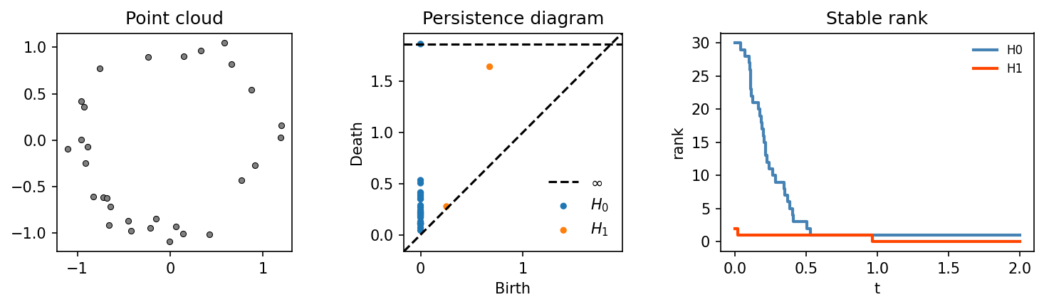
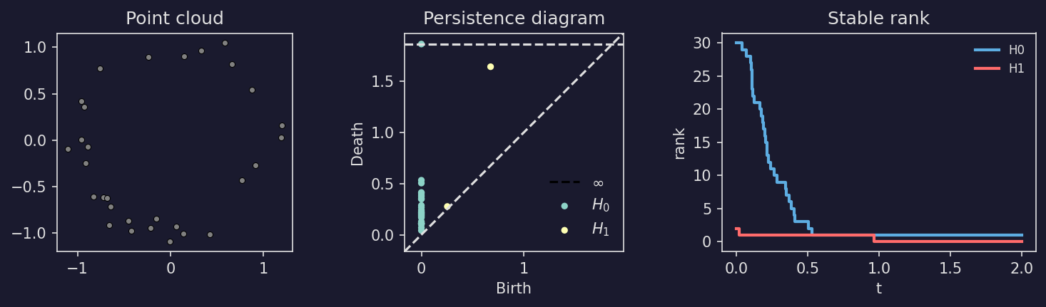
• The (1d) stable rank counts, for each threshold \(t\), how many bars have length at least \(t\) [1][2][3].

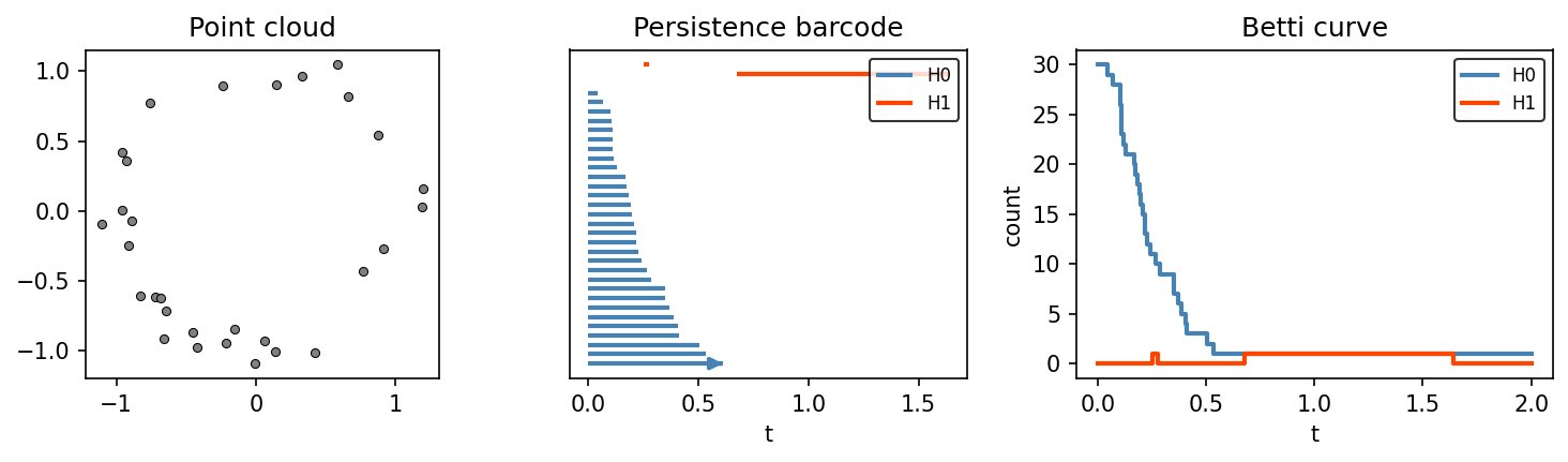
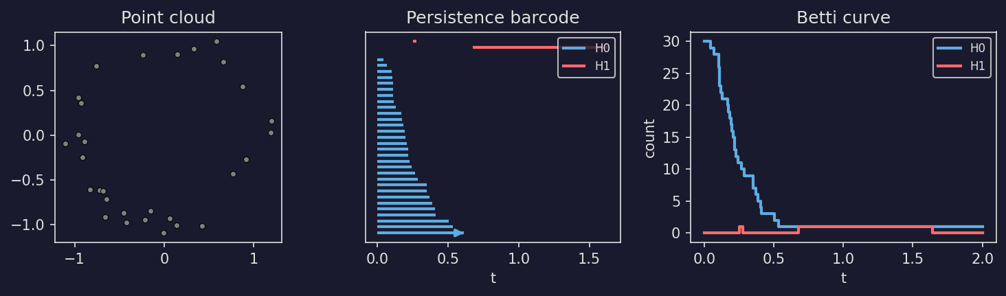
• The Betti curve counts, for each filtration value \(t\), how many bars are alive at \(t\) (see, e.g., [4][5]).

• The accumulated persistence function (APF) sums, for each mean age \(m\), the lifetimes of all bars whose midpoint is at most \(m\) [6].

Because these summaries are PCFs, they fit naturally into masspcf’s tensor framework, enabling efficient computation of distances and means over collections of barcodes.

The pipeline

A typical TDA workflow in masspcf follows three steps:

1. Point clouds – Organize your data into a tensor of point clouds

2. Barcodes – Compute persistent homology to get persistence barcodes

3. Functional summaries – Convert barcodes to PCFs (stable ranks, Betti curves, APFs, etc.) for further analysis

Point clouds  ──>  Barcodes  ──>  Functional summaries (PCFs)
                                       │
                                       ├──  distances (pdist)
                                       ├──  means (mean)
                                       └──  norms (lp_norm)

Step 1: Point clouds

Point clouds are stored in PointCloudTensor. Each element of the tensor is a point cloud, represented internally as an \(n \times d\) numeric array where \(n\) is the number of points and \(d\) is the ambient dimension.

Create a tensor and assign point clouds as NumPy arrays:

import masspcf as mpcf
import numpy as np

# A tensor that will hold 5 point clouds
pclouds = mpcf.zeros((5,), dtype=mpcf.pcloud64)

# Assign random point clouds (varying number of points, 3-dimensional)
for i in range(5):
    n_points = np.random.randint(20, 100)
    pclouds[i] = np.random.randn(n_points, 3)

Point clouds in the same tensor can have different numbers of points and, in principle, different dimensions, though in practice it is most common for all point clouds to share the same ambient dimension.

Higher-dimensional tensors work as well:

# A 10 x 20 grid of point clouds
pclouds = mpcf.zeros((10, 20), dtype=mpcf.pcloud64)

Step 2: Computing persistent homology

compute_persistent_homology() takes a tensor of point clouds and returns a tensor of persistence barcodes. Barcode computation is performed using Ripser [7] under the hood:

from masspcf import persistence as mpers

bcs = mpers.compute_persistent_homology(pclouds, max_dim=1)

The max_dim parameter controls the highest homology dimension computed. With max_dim=1, the function computes \(H_0\) (connected components) and \(H_1\) (loops).

The output tensor has one extra dimension appended, of size max_dim + 1. For example:

• Input shape (5,) with max_dim=1 produces output shape (5, 2)

• Input shape (10, 20) with max_dim=2 produces output shape (10, 20, 3)

To access the \(H_n\) barcode for a specific point cloud, index with the point cloud’s position followed by n:

bc_H0 = bcs[3, 0]   # H0 barcode of point cloud 3
bc_H1 = bcs[3, 1]   # H1 barcode of point cloud 3

Each element is a Barcode object.

Input flexibility

compute_persistent_homology also accepts:

• A single FloatTensor (interpreted as a single point cloud)

• A plain NumPy array (interpreted as a single point cloud)

• A DistanceMatrix (precomputed pairwise distances for a single data set)

• A DistanceMatrixTensor (a tensor of precomputed distance matrices)

# From a NumPy array directly
points = np.random.randn(50, 3)
bcs = mpers.compute_persistent_homology(points, max_dim=1)

When the input is a distance matrix, the distance_type parameter is ignored because distances are already provided:

from scipy.spatial.distance import pdist, squareform
import masspcf as mpcf
from masspcf import persistence as mpers

points = np.random.randn(50, 3)
D = squareform(pdist(points))

dm = mpcf.DistanceMatrix(50, dtype=mpcf.float64)
for i in range(50):
    for j in range(i):
        dm[i, j] = D[i, j]

bcs = mpers.compute_persistent_homology(dm, max_dim=1)

Options

The function supports the following options:

• distance_type – The distance metric used between points. Currently only DistanceType.Euclidean (the default). Ignored when the input is a distance matrix.

• complex_type – The simplicial complex construction. Currently only ComplexType.VietorisRips (the default).

• reduced – If True, compute reduced homology. If False (the default), an essential [0, inf) bar is added to \(H_0\) representing the single connected component that never dies. This matches the convention used by most TDA textbooks.

• verbose – Print progress information (default False).

Step 3: Functional summaries

Persistence barcodes can be converted to piecewise constant functions for downstream analysis. Because the results are PCFs, they fit naturally into masspcf’s tensor framework, enabling distances, means, and norms.

Stable ranks

barcode_to_stable_rank() converts barcodes into stable rank PCFs. The stable rank counts, for each threshold \(t\), the number of bars with length (death minus birth) strictly greater than \(t\) [1]:

sranks = mpers.barcode_to_stable_rank(bcs)

The output tensor has the same shape as the input.

Show code

def plot_tda_pipeline(h0_color="steelblue", h1_color="orangered"):
    from masspcf import persistence as mpers
    from masspcf.plotting import plot_barcode

    # 1. Noisy circle (clear H1 topology)
    rng = np.random.RandomState(10)
    theta = rng.uniform(0, 2 * np.pi, 30)
    r = 1.0 + rng.normal(0, 0.15, 30)
    points = np.column_stack([r * np.cos(theta), r * np.sin(theta)]).astype(np.float64)

    # 2. Compute persistent homology
    bcs = mpers.compute_persistent_homology(points, max_dim=1, verbose=False)
    bc_h0, bc_h1 = bcs[0], bcs[1]

    # 3. Convert to stable rank
    sranks = mpers.barcode_to_stable_rank(bcs)

    fig, (ax1, ax2, ax3) = plt.subplots(1, 3, figsize=(10, 3),
                                         gridspec_kw={"width_ratios": [1, 1, 1.2]})

    # Left: point cloud
    ax1.scatter(points[:, 0], points[:, 1], s=15, color="grey", edgecolors="black",
                linewidths=0.5)
    ax1.set_aspect("equal")
    ax1.set_title("Point cloud")

    # Middle: persistence diagram (via persim)
    import persim
    persim.plot_diagrams(
        [np.asarray(bc_h0), np.asarray(bc_h1)],
        ax=ax2, legend=True, show=False,
    )
    legend = ax2.get_legend()
    legend.get_frame().set_alpha(0)
    fg = ax2.xaxis.label.get_color()
    for text in legend.get_texts():
        text.set_color(fg)
    for line in ax2.get_lines():
        line.set_color(fg)
    ax2.set_title("Persistence diagram")

    # Right: stable rank
    plotpcf(sranks[0], ax=ax3, max_time=2, color=h0_color, linewidth=2,
            label="H0")
    plotpcf(sranks[1], ax=ax3, max_time=2, color=h1_color, linewidth=2,
            label="H1")
    ax3.set_xlabel("t")
    ax3.set_ylabel("rank")
    ax3.set_title("Stable rank")
    leg3 = ax3.legend(fontsize=8)
    leg3.get_frame().set_alpha(0)
    for text in leg3.get_texts():
        text.set_color(fg)

    fig.tight_layout(w_pad=1.5)
    return fig

Betti curves

barcode_to_betti_curve() converts barcodes into Betti curves. The Betti curve counts, for each filtration value \(t\), the number of bars alive at \(t\) (i.e., bars with birth \(\leq t <\) death):

bettis = mpers.barcode_to_betti_curve(bcs)

The output tensor has the same shape as the input.

Show code

def plot_betti_pipeline(h0_color="steelblue", h1_color="orangered"):
    from masspcf import persistence as mpers
    from masspcf.plotting import plot_barcode

    # 1. Noisy circle
    rng = np.random.RandomState(10)
    theta = rng.uniform(0, 2 * np.pi, 30)
    r = 1.0 + rng.normal(0, 0.15, 30)
    points = np.column_stack([r * np.cos(theta), r * np.sin(theta)]).astype(np.float64)

    # 2. Compute persistent homology
    bcs = mpers.compute_persistent_homology(points, max_dim=1, verbose=False)
    bc_h0, bc_h1 = bcs[0], bcs[1]

    # 3. Convert to Betti curves
    bettis = mpers.barcode_to_betti_curve(bcs, verbose=False)

    fig, (ax1, ax2, ax3) = plt.subplots(1, 3, figsize=(10, 3),
                                         gridspec_kw={"width_ratios": [1, 1, 1.2]})

    # Left: point cloud
    ax1.scatter(points[:, 0], points[:, 1], s=15, color="grey",
                edgecolors="black", linewidths=0.5)
    ax1.set_aspect("equal")
    ax1.set_title("Point cloud")

    # Middle: persistence barcode
    y = plot_barcode(bc_h0, ax=ax2, color=h0_color, linewidth=2, label="H0")
    plot_barcode(bc_h1, ax=ax2, y_offset=y + 1, color=h1_color, linewidth=2,
                 label="H1")
    ax2.set_yticks([])
    ax2.set_xlabel("t")
    ax2.set_title("Persistence barcode")
    ax2.legend(fontsize=8)

    # Right: Betti curves
    plotpcf(bettis[0], ax=ax3, max_time=2, color=h0_color, linewidth=2,
            label="H0")
    plotpcf(bettis[1], ax=ax3, max_time=2, color=h1_color, linewidth=2,
            label="H1")
    ax3.set_xlabel("t")
    ax3.set_ylabel("count")
    ax3.set_title("Betti curve")
    ax3.legend(fontsize=8)

    fig.tight_layout(w_pad=1.5)
    return fig

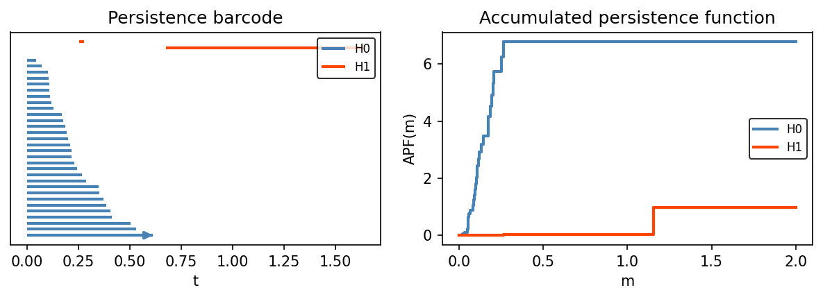
Accumulated persistence functions

barcode_to_accumulated_persistence() converts barcodes into accumulated persistence functions (APFs) [6]. For each mean age \(m\), the APF sums the lifetimes of all bars whose midpoint is at most \(m\):

\[\mathrm{APF}(m) = \sum_{i=1}^{N} \ell_i \, \mathbf{1}(m_i \leq m)\]

where \(N\) is the number of bars, \(\ell_i = d_i - b_i\) is the lifetime, \(m_i = (b_i + d_i)/2\) is the midpoint of bar \(i\), and \(\mathbf{1}(\cdot)\) is the indicator function.

from masspcf import persistence as mpers

apfs = mpers.barcode_to_accumulated_persistence(bcs)

Show plotting code

def plot_apf_example(h0_color="steelblue", h1_color="orangered"):
    from masspcf import persistence as mpers
    from masspcf.plotting import plot_barcode

    # Noisy circle
    rng = np.random.RandomState(10)
    theta = rng.uniform(0, 2 * np.pi, 30)
    r = 1.0 + rng.normal(0, 0.15, 30)
    points = np.column_stack([r * np.cos(theta), r * np.sin(theta)]).astype(np.float64)

    bcs = mpers.compute_persistent_homology(points, max_dim=1, verbose=False)
    bc_h0, bc_h1 = bcs[0], bcs[1]
    apfs = mpers.barcode_to_accumulated_persistence(bcs, verbose=False)

    fig, (ax1, ax2) = plt.subplots(1, 2, figsize=(8, 3))

    # Left: barcode
    y = plot_barcode(bc_h0, ax=ax1, color=h0_color, linewidth=2, label="H0")
    plot_barcode(bc_h1, ax=ax1, y_offset=y + 1, color=h1_color, linewidth=2,
                 label="H1")
    ax1.set_yticks([])
    ax1.set_xlabel("t")
    ax1.set_title("Persistence barcode")
    ax1.legend(fontsize=8)

    # Right: APF
    plotpcf(apfs[0], ax=ax2, max_time=2, color=h0_color, linewidth=2, label="H0")
    plotpcf(apfs[1], ax=ax2, max_time=2, color=h1_color, linewidth=2, label="H1")
    ax2.set_xlabel("m")
    ax2.set_ylabel("APF(m)")
    ax2.set_title("Accumulated persistence function")
    ax2.legend(fontsize=8)

    fig.tight_layout(w_pad=1.5)
    return fig

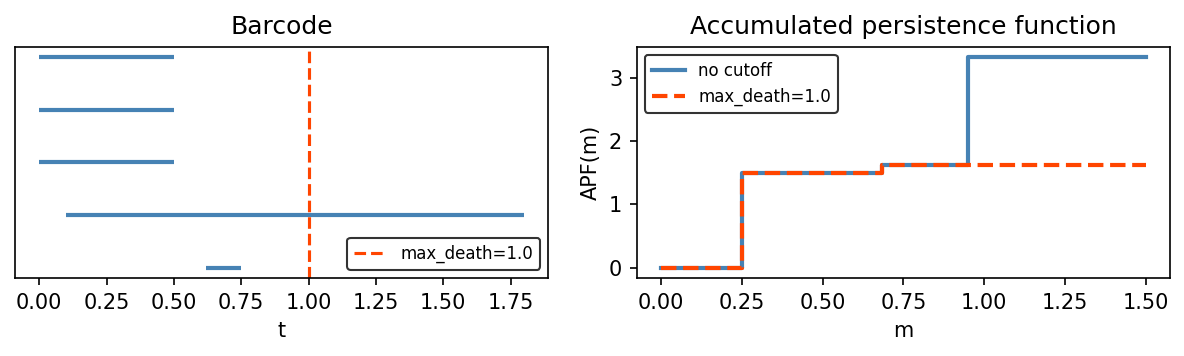
An optional max_death parameter excludes bars whose death time exceeds a given threshold. This corresponds to Equation (2) in [6], where a filtration cutoff \(T\) limits the computation to bars with \(d_i \leq T\):

apfs = mpers.barcode_to_accumulated_persistence(bcs, max_death=25.0)

Show plotting code

def plot_apf_max_death(color1="steelblue", color2="orangered"):
    from masspcf.persistence import Barcode, barcode_to_accumulated_persistence
    from masspcf.plotting import plot_barcode

    bc = Barcode(np.array([
        [0.0, 0.5], [0.0, 0.5], [0.0, 0.5],
        [0.62, 0.75], [0.1, 1.8],
    ], dtype=np.float64))

    apf_all = barcode_to_accumulated_persistence(bc)
    apf_cut = barcode_to_accumulated_persistence(bc, max_death=1.0)

    fig, (ax1, ax2) = plt.subplots(1, 2, figsize=(8, 2.5))

    # Left: barcode with cutoff line
    plot_barcode(bc, ax=ax1, color=color1, linewidth=2)
    ax1.axvline(1.0, color=color2, linestyle="--", linewidth=1.5, label="max_death=1.0")
    ax1.set_yticks([])
    ax1.set_xlabel("t")
    ax1.set_title("Barcode")
    ax1.legend(fontsize=8, loc="lower right")

    # Right: APF with and without cutoff
    plotpcf(apf_all, ax=ax2, max_time=1.5, color=color1, linewidth=2,
            label="no cutoff")
    plotpcf(apf_cut, ax=ax2, max_time=1.5, color=color2, linewidth=2,
            linestyle="--", label="max_death=1.0")
    ax2.set_xlabel("m")
    ax2.set_ylabel("APF(m)")
    ax2.set_title("Accumulated persistence function")
    ax2.legend(fontsize=8)

    fig.tight_layout(w_pad=1.5)
    return fig

Using functional summaries

Since stable ranks and Betti curves are PCFs, they are stored in PCF tensors and support all of masspcf’s standard operations:

import masspcf as mpcf
from masspcf.plotting import plot as plotpcf
import matplotlib.pyplot as plt

# Plot the H1 stable ranks
plotpcf(sranks[:, 1])
plt.title('H1 stable ranks')
plt.show()

# Compute distances between H1 stable ranks
D = mpcf.pdist(sranks[:, 1], verbose=False)

# Compute the mean H1 stable rank
avg = mpcf.mean(sranks[:, 1], dim=0)

Complete example

The following example creates a multidimensional tensor of random point clouds, computes persistent homology, converts to stable ranks, and visualizes the result:

import masspcf as mpcf
from masspcf import persistence as mpers
from masspcf.plotting import plot as plotpcf
import numpy as np
import matplotlib.pyplot as plt

shape = (10, 20)
pcloud_dim = 4

# Create and fill point cloud tensor
pclouds = mpcf.zeros(shape, dtype=mpcf.pcloud64)
for i in range(shape[0]):
    for j in range(shape[1]):
        n_points = np.random.randint(20, 100)
        pclouds[i, j] = np.random.randn(n_points, pcloud_dim)

# Compute persistent homology (H0 and H1)
bcs = mpers.compute_persistent_homology(pclouds, max_dim=1)
print(bcs.shape)   # (10, 20, 2)

# Convert to stable ranks
sranks = mpers.barcode_to_stable_rank(bcs)
print(sranks.shape) # (10, 20, 2)

# Plot H1 stable ranks for the first row of point clouds
plotpcf(sranks[0, :, 1])
plt.title('H1 stable ranks for pclouds[0, :, :]')
plt.show()

# Distance matrix between H1 stable ranks in the first row
D = mpcf.pdist(sranks[0, :, 1], verbose=False)

The Barcode class

Individual barcodes are represented by Barcode. A barcode can be constructed from an \(n \times 2\) NumPy array of (birth, death) pairs:

from masspcf.persistence import Barcode

bc = Barcode(np.array([[0.0, 1.5],
                        [0.2, 3.0],
                        [0.5, 0.8]]))

You can also convert a single barcode to a stable rank:

from masspcf.persistence import barcode_to_stable_rank

sr = barcode_to_stable_rank(bc)
# sr is a Pcf

References

[1] (1,2)

Wojciech Chachólski and Henri Riihimäki. Metrics and stabilization in one parameter persistence. SIAM Journal on Applied Algebra and Geometry, 4(1):69–98, 2020. doi:10.1137/19M1243932.

[2]

Oliver Gäfvert and Wojciech Chachólski. Stable invariants for multiparameter persistence. 2021. arXiv:1703.03632.

[3]

Martina Scolamiero, Wojciech Chachólski, Anders Lundman, Ryan Ramanujam, and Sebastian Öberg. Multidimensional persistence and noise. Foundations of Computational Mathematics, 17:1367–1406, 2017. doi:10.1007/s10208-016-9323-y.

[4]

Yuhei Umeda. Time series classification via topological data analysis. Information and Media Technologies, 12:228–239, 2017. doi:10.11185/imt.12.228.

[5]

Frédéric Chazal and Bertrand Michel. An introduction to topological data analysis: fundamental and practical aspects for data scientists. Frontiers in Artificial Intelligence, 2021. doi:10.3389/frai.2021.667963.

[6] (1,2,3)

Christophe A. N. Biscio and Jesper Møller. The accumulated persistence function, a new useful functional summary statistic for topological data analysis, with a view to brain artery trees and spatial point process applications. Journal of Computational and Graphical Statistics, 28(3):671–681, 2019. doi:10.1080/10618600.2019.1573686.

[7]

Ulrich Bauer. Ripser: efficient computation of Vietoris–Rips persistence barcodes. Journal of Applied and Computational Topology, 5:391–423, 2021. doi:10.1007/s41468-021-00071-5.